Galaxy Evolution
Published 2025-06-XX. [This page is still under construction. It will be completed once I have conquered functional analysis.]
Introduction
The Subaru Prime Focus Spectrograph at the Mauna Kea observatory in Hawai'i seeks to answer the following question: What aspects of large-scale cosmological structure drive the formation and evolution of galaxies?
Researchers from all over the world are working together to construct a first-of-its-kind instrument that can conduct a spectrographic survey "large enough" to precisely identify these causal relationships. Its observations will test our theories of dark matter, illuminate the life cycles of black holes, and trace "reionization" — the moment when the first stars flooded space with ultraviolet light, lifting the fog of the cosmic "dark ages."
Problem
For every night of scheduled observations, the PFS will conduct some small number of exposures $T = 42$, during which each of $K = 2394$ fibers on the instrument will observe a galaxy. Each of $I = 338900$ galaxies are grouped by intrinsic astrophysical properties into classes, and a galaxy's class determines the integration time (i.e. number of exposures) required for it to be completely observed. Notably, any given fiber has access to some, but not necessarily all, galaxies.
Here is the principal question which I and my advisor, Peter Melchior, seek to address:
Given the global objective of balancing the proportion of completed galaxies per class, how can we optimally make local assignments of fibers to galaxies during each exposure?
Explicitly, suppose we denote $\mathcal{I}$ the set of galaxies, $\mathcal{K}$ the set of fibers, and $\mathcal{L}$ the set of exposures. Let the galaxies be partitioned into $M$ classes $\{\Theta_m\}_{m \in \mathcal{M}}$, each with $N_m := |\Theta_m|$ galaxies, based on their shared required observation time $T_m$. Concretely, the problem we'd like to solve (henceforth denoted $\Lambda_1$) is
where $\mathcal{X}$ is the characteristic function. It has an intuitive interpretation, despite its technical representation:
- The scientific objective is an "equitable" distribution among the galaxy classes. It seeks to optimize the minimum fraction of galaxies completed in each class $m$ (i.e. $n_m / N_m$, where $n_m$ is the number of galaxies in $\Theta_m$ which receive at least $T_m$ observation time), across all classes.
- The first constraint asks that each fiber $k$ only observes a predefined subset of galaxies $\Psi_k \subseteq \mathcal{I}$.
- The second constraint asks that in each exposure, there is at most one fiber observing each galaxy.
- The third constraint asks that in each exposure, each fiber observes at most one galaxy.
This combinatorial optimization is extremely hard; in fact, it is NP-hard. Given the high-dimensional nature of the data (there are $IKL\sim \mathcal{O}(10^{10})$ binary decision variables!), brute force is effectively intractable. Instead, we'll need some more powerful tools with the right architecture to exploit this problem's discrete structure.
What are MPNNs?
Message-Passing Neural Networks (MPNNs), introduced by Gilmer et.
al. at ICML 2017 (and later generalized
in Battaglia et. al.'s 2018 graph-nets paper)
are a unified framework for interpreting learning on graphs. Let $G=(V,E)$ be an input graph represented by
node features $\mathbf{h}_v^{(0)}$ and edge features $\mathbf{e}_{uv}$ for $u, v \in V$. Then learning
proceeds through a sequence of $T$ discrete message-passing layers. In each layer $t$:
- Message Phase: for every edge $(u, v) \in E$, generate the message $$ \mathbf{m}_{uv}^{(t)} = M^{(t)}(\mathbf{h}_u^{(t-1)}, \mathbf{h}_v^{(t-1)}, \mathbf{e}_{uv}) $$ where $M^{(t)}$ is a learnable (often neural) function shared across edges.
- Aggregation Phase: each node $v \in V$ aggregates incoming messages with a permutation-invariant operator $\phi$ such as a sum, mean, or max: $$ \mathbf{m}_v^{(t)} = \phi_{u \in \mathcal{N}(v)} \mathbf{m}_{uv}^{(t)} $$ where $\mathcal{N}(\cdot)$ represents the neighborhood of its input (i.e., all connected objects). Permutation-invariance is critical so that the network doesn't associate the arbitrary ordering of the nodes as meaningful information.
- Update Phase: the node state is updated via another learnable function $U^{(t)}$: $$ \mathbf{h}_v^{(t)} = U^{(t)}(\mathbf{h}_v^{(t-1)}, \mathbf{m}_v^{(t)}) $$
After $T$ rounds, the graph-level or node-level readout (e.g., pooling or attention) produces task-specific predictions, which can be used to calculate the objective and loss.
Class-Level Message-Passing
Graph Modeling
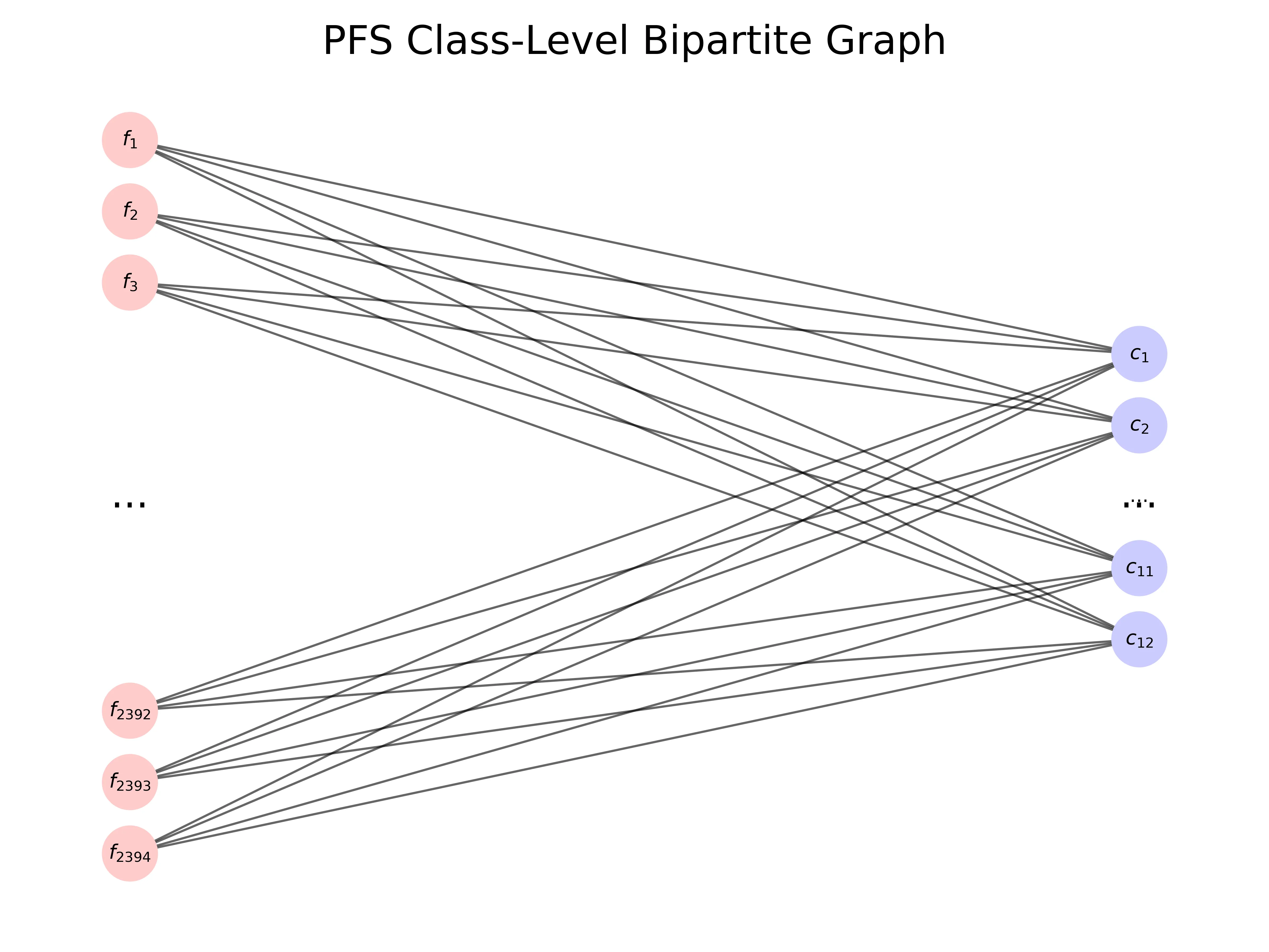
Since the goal of $\Lambda_1$ is to assign each fiber to a particular galaxy target during a given exposure $t$, the natural structure of the problem is bipartite. One way to reduce the dimensionality of the problem comes from looking at galaxy classes, rather than individual galaxies. Let's take a look at properties of the classes:
| $C_1$ | $C_2$ | $C_3$ | $C_4$ | $C_5$ | $C_6$ | $C_7$ | $C_8$ | $C_9$ | $C_{10}$ | $C_{11}$ | $C_{12}$ | |
|---|---|---|---|---|---|---|---|---|---|---|---|---|
| $T_m$ | 2 | 2 | 2 | 12 | 6 | 6 | 12 | 6 | 3 | 6 | 12 | 8 |
| $N_m$ | 68200 | 69300 | 96300 | 14400 | 22000 | 8300 | 14000 | 22000 | 7400 | 4500 | 2800 | 9700 |
Since there are only $M = 12$ classes, while there are $I = \sum_{m \in \mathcal{M}} N_m = 338900$ galaxies, constructing our graph with fibers and classes reduces the number of nodes in the bipartite graph by over a factor of a hundred!
The construction of our graph, then, will be as follows:
- The left part $\mathcal{K}$ will represent fiber nodes.
- The right part $\mathcal{M}$ will represent class nodes.
The remaining question, then, is what the connectivity of the bipartite graph will be, and to what extent this model impacts correctness. To that end, the following (empirically true!) assumption will be useful:
Galaxies are uniformly distributed throughout the fibers' fields of view.
An important consequence of this assumption is that most galaxies will be only observable by exactly one fiber, and furthermore that each fiber will have an abundance of galaxies to observe from every class, should it choose to do so. As a direct result, we can now fully describe our graph by specifying:
- The graph connectivity will be complete.
The point of this graph construction is that every fiber will predict a weight for every class, denoting the number of galaxies from that class it will observe. Because our objective depends on class-completion, not individual galaxies, and is independent of the order of observation, this collection of weights will specify a feasible solution.
In reality, there will be an intra-class ranking of galaxies that we can use to select galaxies from each class, and generally for stability we ought to complete "long-run" — large $T_m$ — targets first. But the point is that once we have the per-fiber class numbers, we may further tune these parameters to find a close-to-optimal solution.
Note that because of our assumption that each galaxy is observable by exactly one fiber, and also due to the abundance of galaxies relative to fiber-exposures ($I\gg KL$), we can be assured that any galaxy which fiber $k$ chooses to observe will be distinct from any other galaxy which fiber $k'$ chooses to observe.
So, onto the engineering front! How can we turn this graph model into an MPNN?
The Lagrangian
Our immediate task is to define a loss function. The Lagrangian that we'll construct should:
- Reflect our modeling choice of optimizing the number of galaxies per class per fiber $n_{km}$ rather than the binary variables $t_{ikl}$.
- Replace the discrete aspects (characteristic function, hard-counts $n_{km}$) with smooth relaxations, so that the loss is differentiable.
The first requirement can be met by formalizing our prior discussion of the graph model:
That's a lot less scary than $\Lambda_1$! To meet the second requirement of smoothness, though, the gradients are more meaningful if we reformulate in terms of the times that each fiber will provide each class, $t_{km} := n_{km} T_m$:
Here, $\{f_\alpha : \mathbb{R} \to \mathbb{R}\}_{\alpha \geq 0}$ is a family of functions with the following property: $f_\alpha \to \text{id}$ as $\alpha \to 0^+$, while $f_\alpha \to \lfloor \cdot \rfloor$ as $\alpha \to \infty$. During training, we'll start by relaxing the parameter $\alpha = 0$ (no discretization) and then increase $\alpha$ to a desirable sharpness.
The version of $f_\alpha$ we'll use is graphed below (the motivation comes from complex analysis, explored below). Try pressing the "play" button to automatically vary $\alpha$ from $0$ to $20$. Notice that even at $\alpha = 10$, the approximation to the floor function is rather good.
Therefore our Lagrangian loss function is
$$ L(t_{11}, \dots, t_{KM}) = - \min_{m \in \mathcal{M}} \left\{ N_m^{-1} \sum_{k \in \mathcal{K}} f_\alpha(t_{km} T_m^{-1}) \right\} + w \cdot p\left(\sum_{m \in \mathcal{M}} t_{km} - T \right) $$ where $p = \operatorname*{LeakyReLU}^2$ is a penalty function to (smoothly) penalize overtime and $w \geq 0$ is a weight, and $$ f_{\alpha}(x) = x + \frac{1}{\pi} \arctan \left( \frac{e^{-1/\alpha} \sin(2\pi x)}{1 - e^{-1/\alpha}\cos(2\pi x)} \right) - \frac{1}{\pi} \arctan \left( \frac{e^{-1/\alpha}}{1-e^{-1/\alpha}} \right) $$Now, we're almost at the crux of this problem: the Message-Passing Layers themselves! We'll motivate the $f_\alpha$ and then discuss what messages are being passed in our network.
Softfloor Construction (Optional)
Our goal is to conjure a family of functions $\{f_\alpha : \mathbb{R} \to \mathbb{R}\}_{\alpha \geq 0}$ such that $\lim_{\alpha \to 0^+} f_\alpha(x) = x$, $\lim_{\alpha \to \infty} f_\alpha(x) = \lfloor x \rfloor$, and $f_\alpha \in C^\infty(\mathbb{R})$ for $\alpha \geq 0$. For a well-articulated exposition on branches, consider Chapter 3 of Stein and Shakarchi's Complex Analysis, from the Princeton Lectures in Analysis series.
Let $\lfloor x \rfloor = x - \{x\}$, where $\{x\} \equiv x \, \operatorname*{mod}\, 1$ denotes the fractional part, which is discontinuous precisely at $\mathbb{Z}$. For each $r \in (0, 1)$ define
$$ \varphi_r(x) := - \frac{1}{\pi} \Im \left( \log(1 - re^{2\pi ix}) \right) \equiv - \frac{1}{\pi} \arctan \left( \frac{r \sin(2\pi x)}{1 - r\cos(2\pi x)} \right) $$where $\log$ denotes the principal branch of the complex logarithm. (The equality follows from unwinding definitions.) Some observations:
- Since $\Re(re^{2\pi ix}) \leq r < 1$, each $\varphi_r$ is smooth.
- As $r \to 1^-$ it can be shown that $\varphi_r(x) \to -\frac{1}{2} + \{x\}$.
- As $r \to 0^+$ continuity implies $\varphi_r(x) \to 0$.
Hence, the natural candidate is $f_r(x) = x - \varphi_r(x) + \psi_r$, where $\psi_r = - \frac{1}{\pi} \arctan(\frac{r}{1-r})$ serves as a constant correction term which tends to $-\frac{1}{2}$ as $r \to 1^-$. Thus the final task is to define a parametrization $r = e^{-1/\alpha}$, since then we have the correct behavior as $\alpha \to 0^+$ and $\alpha \to \infty$.
Message-Passing Layers
TODO.